Dummy Variable Regression is a great tool for business managers. Dummy Variable Regression, for example, provides the means to perform very useful analysis such as Conjoint Analysis. Conjoint analysis quantifies how desirable each product attribute choice is relative to the other available choices for a single product. In other words, the marketer learns which product choices a consumer values most and by how much. In this article and the linked video, you will learn exactly how to perform Conjoint Analysis in Excel using Dummy Variable Regression. That may sound like advanced stuff but it’s really quite a bit simpler than you might imagine.
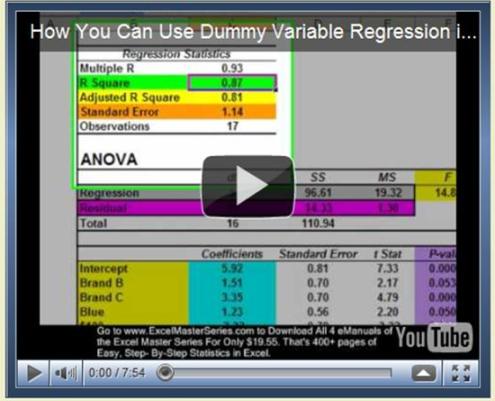
The following video will make the entire procedure of Dummy Variable Regression in Excel to perform Conjoint Analysis much easier to understand:
(Is Your Sound and Internet Connection Turned On?)
Amazon Kindle Users Click here to View Video
The ultimate objective of Conjoint Analysis is quantify the consumer’s degree of liking for each of the choices for one product. The “Utility” of an attribute is the value associated with the consumer’s degree of liking for that choice.
A brief explanation of how Conjoint Analysis and Dummy Variable Regression are used together to arrive at the Utility for each product attribute is as follows and also in the linked video above:
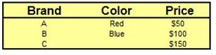
The marketer lists all of the available choices that a consumer has for one product. The marketer starts by listing all of the overall attribute categories such as color and add-ons. The marketer then lists all of the available choices within each attribute category. For example, here the marketer would be listing all available colors and add-ons.
List Of All Product Attributes
The marketer then creates a list of all possible combinations of choices available to the consumer for that one product.
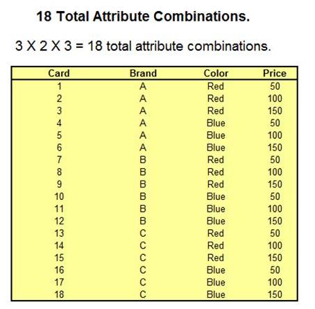
This list of all possible combinations is handed to the consumer. The consumer rates each combination on a scale of 1 (least desirable) to 10 (most desirable).
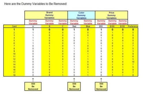
The survey results are arranged so that Dummy Variable Regression can be run on them. Each product choice is assigned its own Dummy Variable and one Dummy Variable from each overall attribute category is removed. This will be explained below and also in more detail in the linked video.
Dummy Variables in a regression are variables that can only assume two values. One Dummy Variable must be created for each product choice.
Dummy Variable Regression is then run on the survey results data.
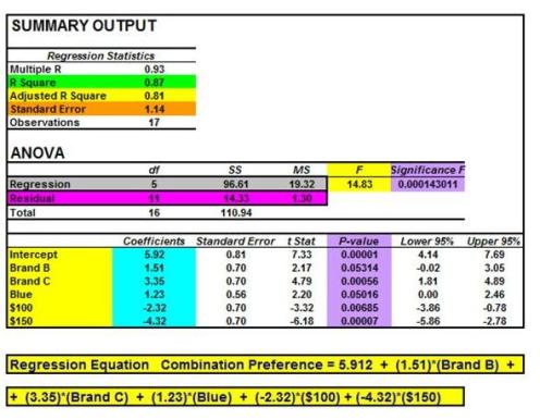
The Utility for each product attribute is derived directly from the coefficients of the resulting regression equation.
Excel Regression Output
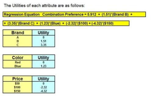
How To Derive The Utilities From the Output
For example, if the product comes only in the colors red and white, There will be a Dummy Variable for red and one for white. The Dummy Variable for the color red can take values of only 1 or 0 because the product will either be red or not.
The same applies for the white Dummy Variable, and all other dummy variables.
When the survey is returned, the survey data is converted into the proper layout for the Regression function in Excel. Each Dummy Variable assigned to a specific attribute will be assigned the value of 0 or 1, depending on whether that attribute was an element of the combination that is currently being rated.
Watching this done in the linked video is probably the easiest way to understand how to do it.
One problem can occur when Dummy Variables are inputs to a regression. The problem of Collinearity or Multicollinearity occurs when any independent variable can be used to predict the value of any other independent variable. For example, if the product comes in only red or white, you can predict whether the product is red if you know whether or not the product is white. This is Collinearity.
Collinearity and Multicollinearity are corrected by removing one Dummy Variable from each choice category. For example, if color choices are red or white, the Dummy Variable for one of those colors would be removed. Collinearity is then solved. You cannot predict whether of not the product is red if you do not know whether the product is white (because the Dummy Variable for white has been removed).
The data can now be run as a regular regression using Excel’s regression tool. The linked video shows how to do this in detail.
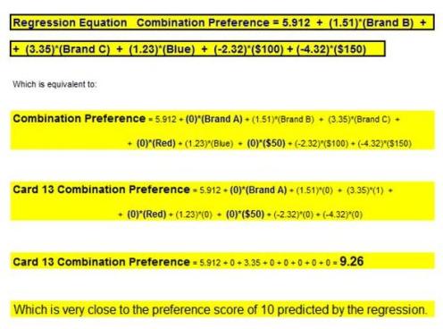
The regression is run and a regression equation is obtained.
The “Utilities” of each of the product choices are set to equal the value of the coefficients of the regression equation. The “Utility” is the degree of liking that the consumer attached to that product choice.
For example, the marketer will find out how important the color red was compared to each of the other product choices during the purchase decision. Utilities of product choices that were associated with the Dummy Variables that were removed to prevent collinearity will be assigned the value of 0.
We now have Utilities for each attribute. Now, the overall attractiveness of a particular combination of choices can be calculated by adding up the individual Utilities associated with the each of the choices. The sum of the Utilities for each combination is the regression’s prediction of consumer’s degree of liking for that combination of product choices.
The removal of the individual Dummy Variables does not affect the accuracy or completeness of the answer. Adding up the Utilities for each combination will produce a figure that will be very close to the consumer’s actual rating for that combination. An example of this is shown in the video.
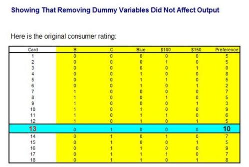
Showing the Regression Equation Predicts Nearly the Same Score as the Customer's Ranking of Card 13, Even Though Dummy Variables Were Removed